Manipulator Simulation
GitHub Repository: MRGilak/manipulator
manipulator
This repo is my object-oriented MATLAB toolbox for simulating a serial manipulator, including kinematics, dynamics, and a few controllers. A 6-DoF robot is used as the running example, but the classes are written to be reusable.
Quick start
Run one of the scripts:
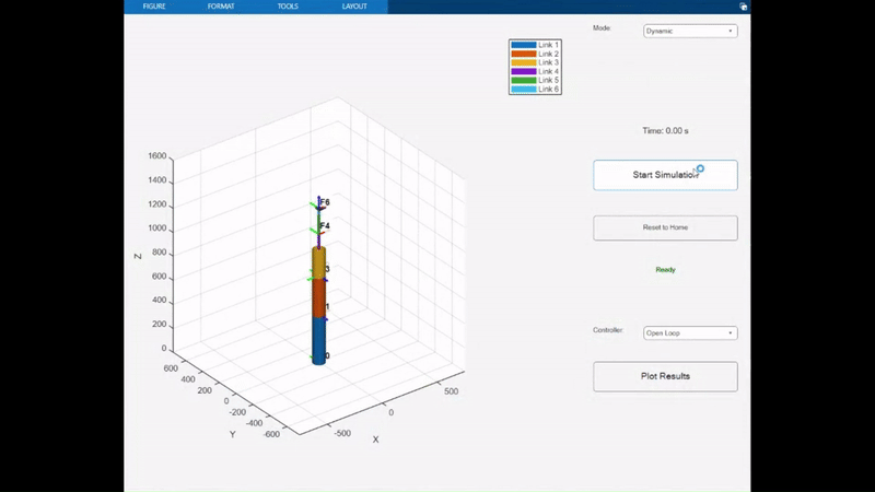
- main.m: joint-space dynamic simulation.
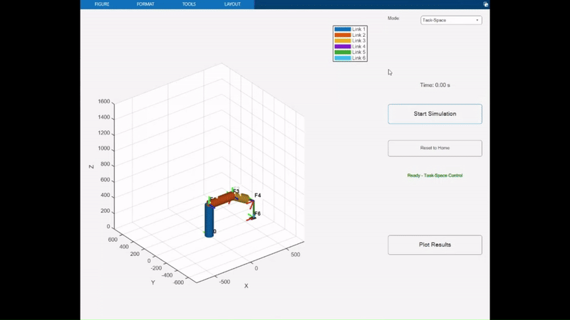
- circle_trajectory.m: task-space circle tracking
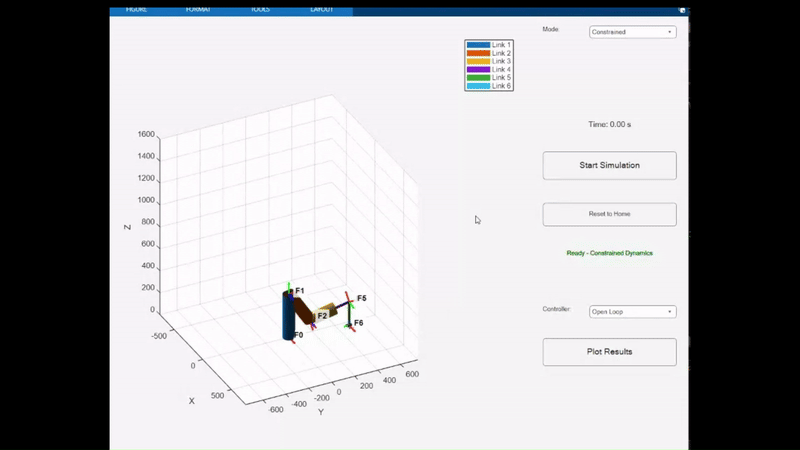
- force_motion_circle.m: constrained dynamics + force-motion control (end-effector constrained against the “floor”).
The following shows the manipulator in action in different cases.
Units and conventions
- Length is in mm.
- Time is in s.
- Default gravity is $g_0 = 9810 mm/s^2$ in Manipulator.
This is a consistent mm–s system. If you set link masses in kg (as in the examples), the implied force unit becomes kg·mm/s^2, i.e. milli-Newtons. That’s why you’ll see things like F_des = 2000 being treated as 2N. Same story for torques (they end up in a scaled mm-based unit).
If you change units, change them everywhere.
Theoretical background
Kinematics (DH)
The kinematics are based on the Denavit–Hartenberg (DH) convention.
The homogeneous transform from frame 0 to frame 1 is
\[H_1^0 = \begin{bmatrix} R_1^0 & d_1^0 \\ 0_{1\times3} & 1 \end{bmatrix},\]where $R_1^0$ is a rotation matrix and $d_1^0$ is a translation vector.
For the 6DoF robot that’s being used in the codes, the DH frames are shown here:
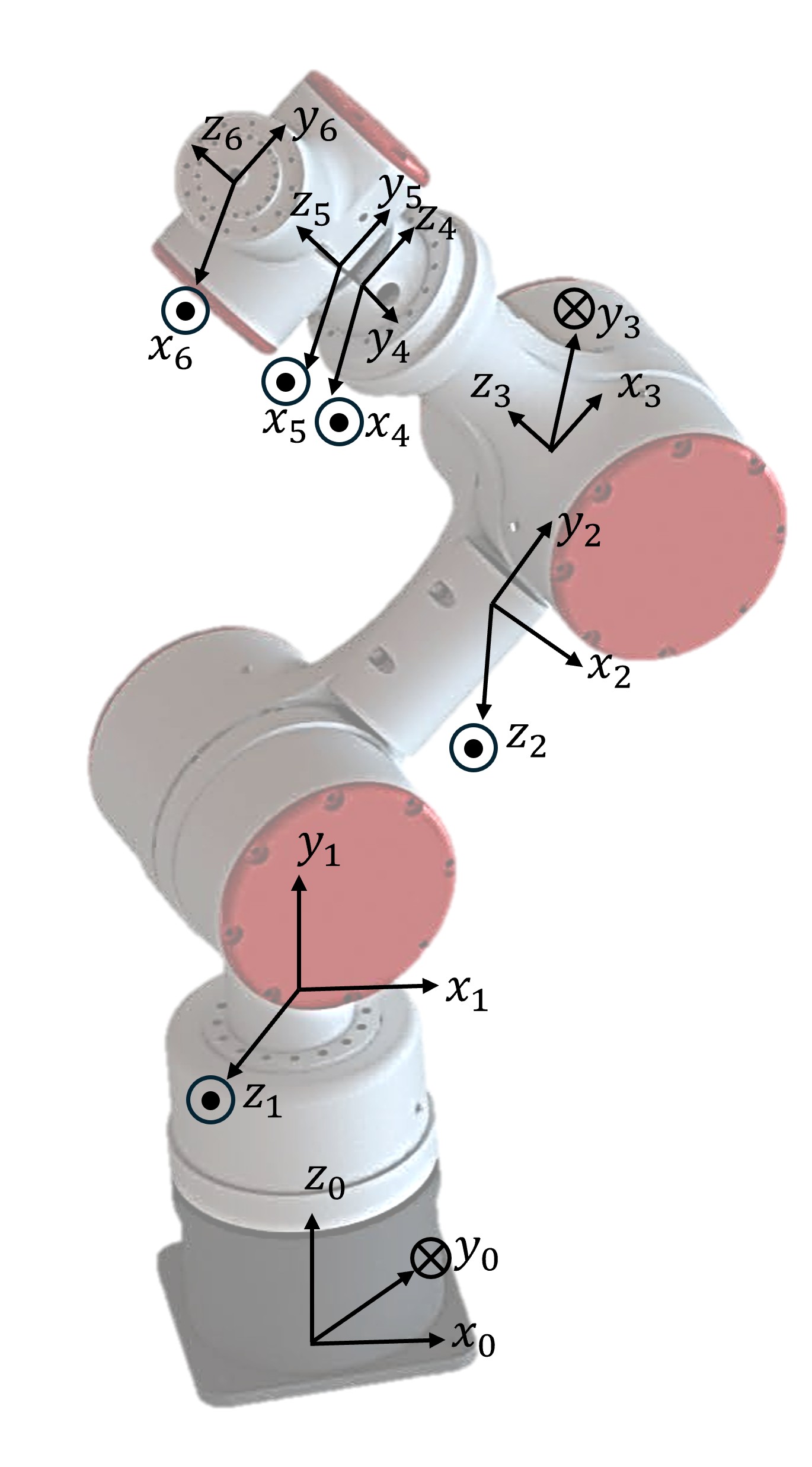
And the parameters here:
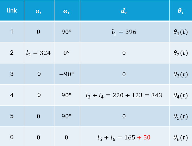
In the code:
Manipulator.dh()builds a single DH transform.Manipulator.fk(frameIdx)multiplies transforms up toframeIdx.
Jacobians
Geometric Jacobian (end-effector)
The geometric Jacobian maps joint angular (or linear) velocities to end-effector linear and angular velocity:
\[\begin{bmatrix} v \\ \omega \end{bmatrix} = J(q)\,\dot q,\]where $J\in\mathbb{R}^{6\times n}$.
In the code:
jacobianOmega(frameIdx)returns $J_\omega$.jacobianLinear(frameIdx)returns $J_v$.jacobian(frameIdx)returns $J = \begin{bmatrix}J_v \ J_\omega\end{bmatrix}$.
COM Jacobians
For dynamics, each link needs a Jacobian at its center of mass (COM). The code builds COM Jacobians and stacks them into one generalized Jacobian (all COMs).
The basic COM mapping used in the code is
\[J_C = \begin{bmatrix} I & S(r_{CD}) \\ 0 & I \end{bmatrix} J_D,\]where $S(\cdot)$ is the skew-symmetric matrix and $r_{CD}$ is the COM offset.
In the code:
jacobianCOM(linkIdx)returns one link’s COM Jacobian.jacobianCOM_all()stacks all COM Jacobians.jacobianCOM_dot(dt)computes a numerical derivative (finite difference).
Dynamics
The dynamics of the robot are as follows:
\[D(q)\ddot q + C(q,\dot q)\dot q + G(q) = \tau.\]In the code:
massMatrix()builds $M$.coriolisMatrix()builds the stacked $S$.gravityVector()builds $g$.inertiaMatrix()returns $D(q)$.coriolisCentrifugalMatrix(dt)returns $C(q,\dot q)$ (numerical $\dot J$).gravityTorque()returns $G(q)$.
Constrained dynamics (environment constraints)
For constrained simulation, the environment provides an environment Jacobian $J_e$ that constrains the end-effector:
\[J_e\,\begin{bmatrix}v\\\omega\end{bmatrix} = 0.\]Since $\begin{bmatrix}v\\omega\end{bmatrix} = J\dot q$, the velocity constraint is
\[J_e\,J\dot q = 0.\]Differentiating gives an acceleration-level constraint:
\[J_e\,J\ddot q + (\dot J_e\,J + J_e\,\dot J)\dot q = 0.\]The constrained equations of motion are solved via an augmented system with $\lambda$:
\[\begin{align} \begin{bmatrix} D & J^T J_e^T \\ J_e J & 0 \end{bmatrix} \begin{bmatrix} \ddot q \\ \lambda \end{bmatrix} = \begin{bmatrix} \tau - C\dot q - G \\ -(\dot J_e\ J + J_e\ \dot J)\dot q \end{bmatrix}. \end{align}\]In the code:
setEnvironmentJacobian(J_e)sets the constraint.environmentJacobianDot(dt)computes $\dot J_e$ numerically.constrainedDynamics(tau, dt)returns $(\ddot q, \lambda, F)$.
The reported contact force is computed as
\[F = J_e^T\lambda.\]Controllers
All controllers are in the Controller class and are selected via controller.type.
Open-Loop
Just outputs zero torque:
\[\tau = 0.\]Useful for sanity-checking the passive dynamics.
Gravity Compensation
Cancels gravity in joint space:
\[\tau = G(q).\]PD
Joint-space PD to a fixed reference:
\[\tau = K_p(q_d - q) - K_d\dot q.\]PD with Gravity Compensation
Adds gravity cancellation to PD:
\[\tau = G(q) + K_p(q_d - q) - K_d\dot q.\]Slotine (tracking)
This is the Slotine controller for manipulators.
Define
\[v = \dot q_d - \Lambda(q - q_d), \qquad \dot v = \ddot q_d - \Lambda(\dot q - \dot q_d), \qquad s = \dot q - v.\]Then
\[\tau = D(q)\dot v + C(q,\dot q) v + G(q) - K s.\]In code, Lambda and K are the gain matrices.
Force-motion (for constrained dynamics)
This controller is meant to be used with Simulation.mode = 'constrained'.
The implemented law is
\[\tau = D(q)\ddot q_d + C(q,\dot q)\dot q_d + G(q) + J(q)^T F_d - K(\dot q - \dot q_d).\]- $F_d\in\mathbb{R}^{6\times1}$ is a desired end-effector force
Actuator saturation
Controller.setSaturation(uMax, uMin) clamps joint torques. You can pass scalars or per-joint vectors.
Code guide
Below is a description of the codes.
Manipulator class
Key properties
- DH:
a,d,alpha,jointType,n. - State:
q,qdot. - History:
q_his,qdot_his,qddot_his,u_his. - Base:
baseT. - Visualization:
visual,graphics. - COM/dynamics:
comOffset,mass,inertia,g0. - Numerical derivatives:
J_prev(shared internal cache). - Trajectory IK cache:
R_d_prev,O_d_prev. - Constraints:
J_e,J_e_prev,lambda_his,F_his.
Kinematics methods
dh(theta, d, a, alpha)dhTransform(i)fk(frameIdx)jacobianOmega(frameIdx)jacobianLinear(frameIdx)jacobian(frameIdx)
COM + dynamics methods
jacobianCOM(linkIdx)jacobianCOM_all()jacobianCOM_dot(dt)massMatrix()coriolisMatrix()gravityVector()inertiaMatrix()inertiaMatrixDot(dt)coriolisCentrifugalMatrix(dt)gravityTorque()
Constraints
setEnvironmentJacobian(J_e)environmentJacobianDot(dt)constrainedDynamics(tau, dt)
IK / differential kinematics
inverseKinematics(R_d, O_d, ...): velocity-level IK (damped least squares). It can use provided derivatives or approximate them numerically.ik(T_desired, q_init, max_iter, tol): position-level IK using iterative damped least squares. It computes an orientation error vialogm().
Utilities + debugging
skew(w),unskew(S)updatePosition(d, v, dt),updateRotation(R, omega, dt),updateTransform(T, v, omega, dt)integrateJointVelocities(dt)checkInertiaMatrixPD(),checkSkewSymmetry(dt)
Visualization
The drawing code is in the same class. The main entry points are:
draw(ax)updateGraphics()
Everything else under that (frames, labels, end-effector styles) is a helper.
Controller class
Properties
type,robot,dt- Desired signals:
qdes,qdotdes,qddotdes - PD gains:
Kp,Kd - Slotine gains:
Lambda,K - Force-motion:
F_des - Saturation:
useSaturation,uMax,uMin
Methods
Controller(robot, type, dt, ...): constructor. Arguments depend ontype.uNext(): computes the torque command based ontype.setSaturation(uMax, uMin)
Note: Robust/Adaptive controllers wil be implemented later, but are not ready at the moment.
Simulation class
Properties
- Objects:
robots,controllers - Time:
time,dt,controlTime - UI:
fig,ax,controls,mode - Trajectory tracking:
trajectoryFunc,useTrajectory,R_prev,O_prev - Histories:
qdes_his,qdotdes_his,O_his,Odes_his,F_des_his
Core workflow
run(...)creates UI/figure (unless headless).- Timers drive the dynamic and velocity modes.
dynamicsTimerCallback()is the core integration loop.
Modes
The UI is mode-based. The main modes you’ll run into are:
manual: sliders for joint positions.velocity: sliders for joint velocities.dynamic: integrates $\ddot{q}$ using the standard dynamics.task-space: dynamic integration plusupdateDesiredFromTrajectory().constrained: usesManipulator.constrainedDynamics()instead of unconstrained dynamics.
Plotting/saving
plotResults()and helpers:plotVariable,plotVariableWithRef,plotEndEffector,plotCircularTrajectory2D.saveResults(filename)andsaveToExcel(filename, results).- Static helpers:
loadAndPlot(...),animateFromData(results),plotVariableStatic(...).
Example scripts
main.m
Joint-space dynamic simulation with a selectable controller.
circle_trajectory.m
Task-space circle tracking. The key parts are:
sim.mode = 'task-space'sim.trajectoryFunc = @(t) ...sim.useTrajectory = true
force_motion_circle.m
Constrained circle on the “floor” with force regulation. It demonstrates:
- Initializing the robot on the constraint manifold (solve IK at $t=0$).
- Setting an environment Jacobian (e.g., constrain end-effector $v_z$).
- Running constrained dynamics + force-motion control.
Notes (practical)
- If you constrain motion, initialize on the constraint. Otherwise the solver will produce very large multipliers $\lambda$ to fight the initial constraint violation.
Manipulator.ik()useslogm()for orientation error. For a 180° rotation you may get a MATLAB warning about the principal logarithm. It’s usually harmless if the IK converges.- The augmented constrained matrix can become ill-conditioned near singular Jacobians. If you hit that, the first fix is almost always better initialization + less aggressive gains.
TODO
- Add complete support for multiple robots (the infrastructure is partly there).
- Add more controllers (robust/adaptive, impedance, etc.).