Active Disturbance Rejection Control
GitHub Repository: MRGilak/Active-Disturbance-Rejection-Controller
This repository contains Python, C++, MATLAB, and Simulink implementation of Active Disturbance Rejection Control with Extended State Observer (ESO), Tracking Differentiator (TD), input delay compensation, control saturation, and support for optional use of the cascaded structure.
I’ve summarized a comprehensive note on the theoretical background of active disturbance rejection controller and tracking differentiators. You can find it in this section (I’ll add the cascaded ADRC documentation as soon as possible).
Note: Important notes for the Python, C++, Matlab, and Simulink implementations are given after the introduction!
New: Cascaded ADRC is now supported for all the environments as well.
Demo
Here are some figures showing the controller in action, in presence of time-varying reference signal, input delay, input saturation, etc.
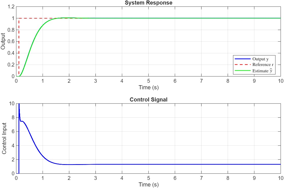
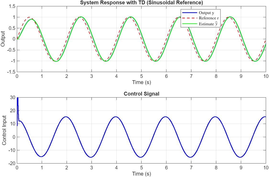
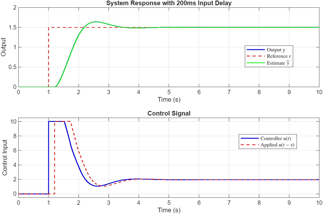
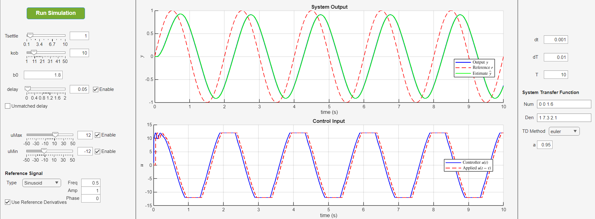
Please pay attention to the following:
Python
Note: Good news! You can install the Python implementation using
pip install adrc
You can look at the project page on Pypi for more information.

Disclaimer: This badge is provided by shields.io. Source analytics dashboard: clickhouse-analytics.metabaseapp.com.
Note: To be able to use all the Python codes, especially the demo script, you need to have the following packages installed:
- numpy
- scipy (only needed for the demo)
- matplotlib (only needed for the demo)
- python-control (only needed for the demo)
Simulink
Discrete controller implementations are available for first and second-order systems in simulink. There is also a continuous-time implementation for second-order systems. Continuous-time first-order systems will be added as well. Please pay attention to the following:
- The model settings in all cases is set to variable step solver. I do encourage using this option, unless there is a specific system you are working with and you know what you are doing.
- In discrete-time simulations, it is necessary that you change the sample time not only where you pass it to the controller, but also in the two or three (depending on the system order) delay blocks that are present in the observer block. I am looking into a way to circumvent this, but for now, you have to change them manually.
- I have added support for first-order and second-order cascaded ADRC as well. You can compare their performance against the standard ADRC in the two simulink files.
- The Simulink files are generated using MATLAB 2025b. If you have an older version and need the files, you can contact me to export them for you. I will add automatic support for older versions as well in the future. You can contact me via email at mrgilak02@gmail.com, but I might not be able to respond quickly due to frequent internet shutdowns in Iran :)
MATLAB
You can take a look at this file to see how the code works.
Note: I have tried to use the same names in MATLAB, Python, and C++; however, I still feel it’s necessary to add proper documentation for each. This is in the TODOs.
- Sample Time: Controller sample time
dTcan differ from simulation time stepdt. The controller should be called at ratedT. - Delay Compensation: Input delay is specified in seconds and internally converted to discrete steps. Delay buffer maintains control history.
- Initialization: Always call
initialize()beforestep(). The controller will throw an error if used uninitialized. - TD Integration: When TD is enabled, it is automatically updated within
step(). Manual reference derivatives can still be provided viavararginto override TD estimates. - State Estimation: Access estimated states via
getEstimatedStates()for monitoring or additional processing.
Theoretical Background
System Representation
Consider an nth-order SISO system:
\[y^{(n)} = f(y, \dot{y}, \ldots, y^{(n-1)}, w(t)) + b_0 u\]where:
- $y$ is the system output
- $u$ is the control input
- $b_0$ is the control gain (nominal)
- $f(\cdot)$ represents the total disturbance (internal dynamics + external disturbances)
- $w(t)$ represents external disturbances
State-Space Form
Define state variables: \(x_1 = y, \quad x_2 = \dot{y}, \quad \ldots, \quad x_n = y^{(n-1)}\)
The system can be written as:
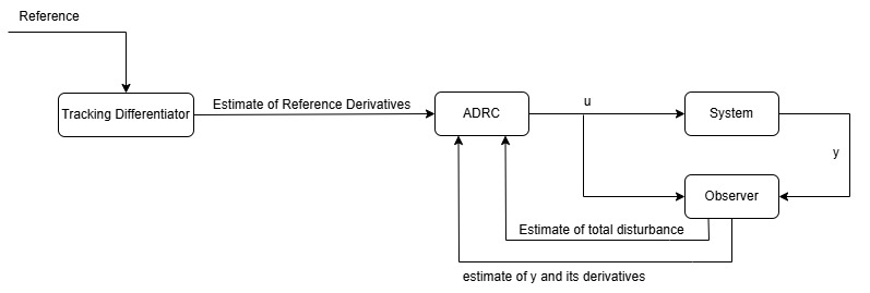
\[\begin{aligned} \dot{x}_1 &= x_2 \\ \dot{x}_2 &= x_3 \\ &\vdots \\ \dot{x}_n &= f + b_0 u \\ y &= x_1 \end{aligned}\]Basically, Active Disturbance Rejection Controller (ADRC) sees the whole system as a multi-integrator plus disturbance. The states are estimated using an observer. Because the total disturbance is estimated as well, the observer is referred to as Extended State Observer (ESO). The diagram below shows the block diagram of ADRC.
Extended State Observer (ESO)
To estimate both the states and the total disturbance $f$, we augment the state vector with $x_{n+1} = f$ (assuming $\dot{f} \approx 0$):
\[\begin{aligned} \dot{x}_1 &= x_2 \\ \dot{x}_2 &= x_3 \\ &\vdots \\ \dot{x}_n &= x_{n+1} + b_0 u \\ \dot{x}_{n+1} &= \dot{f} \approx 0 \\ y &= x_1 \end{aligned}\]In matrix form:
\[\begin{aligned} \dot{\mathbf{x}} &= \mathbf{A} \mathbf{x} + \mathbf{B} u \\ y &= \mathbf{C} \mathbf{x} \end{aligned}\]where:
\[\mathbf{A} = \begin{bmatrix} 0 & 1 & 0 & \cdots & 0 & 0 \\ 0 & 0 & 1 & \cdots & 0 & 0 \\ \vdots & \vdots & \vdots & \ddots & \vdots & \vdots \\ 0 & 0 & 0 & \cdots & 0 & 1 \\ 0 & 0 & 0 & \cdots & 0 & 0 \end{bmatrix}_{(n+1) \times (n+1)}, \quad \mathbf{B} = \begin{bmatrix} 0 \\ 0 \\ \vdots \\ b_0 \\ 0 \end{bmatrix}, \quad \mathbf{C} = \begin{bmatrix} 1 & 0 & \cdots & 0 & 0 \end{bmatrix}\]The ESO is designed as:
\[\dot{\hat{\mathbf{x}}} = \mathbf{A} \hat{\mathbf{x}} + \mathbf{B} u + \mathbf{L}(y - \hat{y})\]where $\mathbf{L} = [l_1, l_2, \ldots, l_{n+1}]^T$ is the observer gain vector.
Observer Gain Selection
The observer gains are selected using bandwidth parameterization. We place all observer poles at $s = -\omega_o$ where $\omega_o$ is the observer bandwidth:
\[\det(sI - (\mathbf{A} - \mathbf{L}\mathbf{C})) = (s + \omega_o)^{n+1}\]For different system orders:
First-order system (n=1):
\[\begin{aligned} l_1 &= 2\omega_o \\ l_2 &= \omega_o^2 \end{aligned}\]Second-order system (n=2):
\[\begin{aligned} l_1 &= 3\omega_o \\ l_2 &= 3\omega_o^2 \\ l_3 &= \omega_o^3 \end{aligned}\]Third-order system (n=3):
\[\begin{aligned} l_1 &= 4\omega_o \\ l_2 &= 6\omega_o^2 \\ l_3 &= 4\omega_o^3 \\ l_4 &= \omega_o^4 \end{aligned}\]Fourth-order system (n=4):
\[\begin{aligned} l_1 &= 5\omega_o \\ l_2 &= 10\omega_o^2 \\ l_3 &= 10\omega_o^3 \\ l_4 &= 5\omega_o^4 \\ l_5 &= \omega_o^5 \end{aligned}\]The observer bandwidth is typically chosen as: \(\omega_o = k_{ob} \cdot \omega_c\)
where $\omega_c = -s_{cl}$ and $s_{cl} = \frac{-4}{T_{settle}}$ (for the first-order system) is the desired closed-loop pole location, and $k_{ob}$ is a multiplier (typically 5-20). $s_{cs}$ is usually selected as to make the closed-loop system critically damped.
Discrete-Time ESO
The continuous ESO is discretized using exact discretization:
\[\mathbf{A}_d = e^{\mathbf{A} \Delta T}\] \[\mathbf{B}_d = \int_0^{\Delta T} e^{\mathbf{A} \tau} d\tau \cdot \mathbf{B} = \mathbf{A}^{-1}(\mathbf{A}_d - \mathbf{I})\mathbf{B}\]For numerical stability, we compute:
\[\mathbf{B}_d = \sum_{i=1}^{n} \frac{(\Delta T)^i}{i!} \mathbf{A}^{i-1} \mathbf{B}\]The discrete observer gains are computed using pole placement in the z-domain. For a pole at $z = e^{s \Delta T}$ where $s = -\omega_o$:
\[z_{eso} = e^{-\omega_o \Delta T}\]The discrete gains $L_d$ are selected such that the characteristic polynomial matches $(z - z_{eso})^{n+1}$.
For n=1:
\[\begin{aligned} L_{d,1} &= 1 - z_{eso}^2 \\ L_{d,2} &= \frac{(1 - z_{eso})^2}{\Delta T} \end{aligned}\]For n=2:
\[\begin{aligned} L_{d,1} &= 1 - z_{eso}^3 \\ L_{d,2} &= \frac{3(1 + z_{eso})(1 - z_{eso})^2}{2\Delta T} \\ L_{d,3} &= \frac{(1 - z_{eso})^3}{\Delta T^2} \end{aligned}\]For n=3:
\[\begin{aligned} L_{d,1} &= 1 - z_{eso}^4 \\ L_{d,2} &= \frac{(1 - z_{eso})^2(11 + z_{eso}(14 + 11z_{eso}))}{6\Delta T} \\ L_{d,3} &= \frac{2(1 - z_{eso})^3(1 + z_{eso})}{\Delta T^2} \\ L_{d,4} &= \frac{(1 - z_{eso})^4}{\Delta T^3} \end{aligned}\]For n=4:
\[\begin{aligned} L_{d,1} &= 1 - z_{eso}^5 \\ L_{d,2} &= \frac{5(1 - z_{eso})^2(1 + z_{eso})(5 + z_{eso}(2 + 5z_{eso}))}{12\Delta T} \\ L_{d,3} &= \frac{5(1 - z_{eso})^3(7 + z_{eso}(10 + 7z_{eso}))}{12\Delta T^2} \\ L_{d,4} &= \frac{5(1 - z_{eso})^4(1 + z_{eso})}{2\Delta T^3} \\ L_{d,5} &= \frac{(1 - z_{eso})^5}{\Delta T^4} \end{aligned}\]The discrete ESO update equation:
\[\hat{\mathbf{x}}[k] = \mathbf{A}_d \hat{\mathbf{x}}[k-1] + \mathbf{B}_d u[k-1] + \mathbf{L}_d (y[k] - \mathbf{C}_d \mathbf{A}_d \hat{\mathbf{x}}[k-1])\]Simplified form:
\[\hat{\mathbf{x}}[k] = (\mathbf{A}_d - \mathbf{L}_d \mathbf{C}_d \mathbf{A}_d) \hat{\mathbf{x}}[k-1] + (\mathbf{B}_d - \mathbf{L}_d \mathbf{C}_d \mathbf{B}_d) u[k-1] + \mathbf{L}_d y[k]\]Control Law
The control law compensates for the estimated disturbance and tracks the reference:
\[u_0 = \frac{1}{b_0} \left[ r^{(n)} - \sum_{i=1}^{n} k_i (r^{(i-1)} - \hat{x}_i) - \hat{x}_{n+1} \right]\]where $r$ is the reference signal and $k_i$ are the state feedback gains.
Equivalently:
\[u_0 = \frac{1}{b_0} \left[ \mathbf{K}^T (\mathbf{r} - \hat{\mathbf{x}}) \right]\]where:
\[\mathbf{r} = \begin{bmatrix} r \\ r^{(1)} \\ \vdots \\ r^{(n-1)} \\ r^{(n)} \end{bmatrix}, \quad \mathbf{K} = \begin{bmatrix} k_1 \\ k_2 \\ \vdots \\ k_n \\ 1 \end{bmatrix}\]Controller Gain Selection
The controller gains are selected by pole placement. All closed-loop poles are placed at $s = -\omega_c$:
\[\det(sI - (\mathbf{A} - \mathbf{B}\mathbf{K}^T)) = (s + \omega_c)^n\]where $\omega_c = \frac{-4}{T_{settle}}$ for a desired settling time $T_{settle}$.
For an nth-order system:
\[k_i = \binom{n}{i} \omega_c^i, \quad i = 1, 2, \ldots, n\]Examples:
For n=2: $k_1 = 2\omega_c$, $k_2 = \omega_c^2$
For n=3: $k_1 = 3\omega_c$, $k_2 = 3\omega_c^2$, $k_3 = \omega_c^3$
Tracking Differentiator (TD)
When reference derivatives are not available, a Tracking Differentiator is used to estimate them from the reference signal. Five TD methods are implemented:
1. Euler-based TD
Low-pass filter with numerical differentiation:
\[\begin{aligned} y_f[k] &= a \cdot y_f[k-1] + (1-a) \cdot r[k] \\ \dot{y}_f[k] &= \frac{y_f[k] - y_f[k-1]}{\Delta T} \end{aligned}\]Parameter: $a \in (0,1)$ (filter coefficient)
2. Time-Optimal Differentiator (TOD)
\[\begin{aligned} \dot{v}_1 &= v_2 \\ \dot{v}_2 &= -r \cdot \text{sign}\left( v_1 - r + \frac{v_2 |v_2|}{2r} \right) \end{aligned}\]Parameter: $r > 0$ (convergence rate)
3. Linear Differentiator (LD)
\[\begin{aligned} \dot{v}_1 &= v_2 - \frac{v_1 - r}{\lambda} \\ \dot{v}_2 &= -\frac{2(v_1 - r)}{\lambda} \end{aligned}\]Parameter: $\lambda > 0$ (bandwidth)
4. Robust Exact Differentiator (RED)
\[\begin{aligned} \dot{v}_1 &= v_2 - \lambda_1 |e|^{0.5} \text{sign}(e) \\ \dot{v}_2 &= -\lambda_2 \text{sign}(e) \end{aligned}\]where $e = v_1 - r$
Parameters: $\lambda_1, \lambda_2 > 0$
5. Improved Nonlinear TD (INTD)
\[\begin{aligned} \dot{v}_1 &= v_2 \\ \dot{v}_2 &= -r^2 \tanh\left( \frac{\beta v_1 - (1-\alpha) r}{\gamma} \right) - r v_2 \end{aligned}\]Parameters: $\alpha \in [0,1]$, $\beta, \gamma, r > 0$
All TDs are integrated using forward Euler with sample time $\Delta T$.
Input Delay Compensation
When the system has input delay $\tau$, the actual plant input is $u(t-\tau)$. The ESO is modified to use the delayed control signal:
\[\hat{\mathbf{x}}[k] = \mathbf{A}_d \hat{\mathbf{x}}[k-1] + \mathbf{B}_d u[k-1-d] + \mathbf{L}_d y[k]\]where $d = \lfloor \tau / \Delta T \rfloor$ is the delay in samples.
The controller computes the current control signal, while the ESO uses the control signal from $d$ steps ago, which is the signal currently affecting the plant.
Control Saturation
When control saturation limits $[u_{min}, u_{max}]$ exist, the control signal is saturated:
\[u = \begin{cases} u_{max} & \text{if } u_0 > u_{max} \\ u_{min} & \text{if } u_0 < u_{min} \\ u_0 & \text{otherwise} \end{cases}\]The saturated control signal $u$ is fed back to the ESO to maintain consistency between the ESO’s prediction and the actual plant input.
This repo is maintained by me. Contributions are welcome as well. —
References
- Han, J. (2009). “From PID to Active Disturbance Rejection Control”. IEEE Transactions on Industrial Electronics.
- Gao, Z. (2006). “Active Disturbance Rejection Control: A Paradigm Shift in Feedback Control System Design”. American Control Conference.
- Herbst, G. (2013). “A Simulative Study on Active Disturbance Rejection Control (ADRC) as a Control Tool for Practitioners”. Electronics.
- Zheng, Q., Gao, Z. (2010). “On Practical Applications of Active Disturbance Rejection Control”. Chinese Control Conference.
- Madoński, R., & Herman, P. (2015). Survey on methods of increasing the efficiency of extended state disturbance observers. ISA transactions, 56, 18-27.