Multi-arm Bandits
#RL #Learning #computer-science
This note is almost entirely based on the book Reinforcement Learning: An Introduction by Sutton. I highly encourage reading the book itself for more detailed information and clear explanations.
Multi-arm bandit is a classic RL example that teaches the basic algorithms. In this note, we take a closer look at this example. The most important feature distinguishing reinforcement learning from other types of learning is that it uses training information that evaluates the actions taken, instead of instructing the learner. Purely evaluative feedback indicates how good the action taken is, but not whether it is the best or the worst action possible.
Problem Statement
Consider the following learning problem: You are faced repeatedly with a choice among $n$ different options, or actions. After each choice you receive a numerical reward chosen from a stationary probability distribution that depends on the action you selected. Your objective is to maximize the expected total reward over some time period. Selecting each action results in an expected or mean reward, called the value of that action. If the value of each action were known, then one would always select the action with highest value; Therefore, we assume we don’t know the action value with certainty.
Exploring vs Exploiting
If you maintain estimates of the action values, then at any time step there is at least one action whose estimated value is greatest. This is called a greedy action. If you select a greedy action, we say that you are exploiting your current knowledge of the values of the actions. If instead you select one of the non-greedy actions, then we say you are exploring. Exploitation is the right thing to do to maximize the expected reward on the one step, but exploration may produce the greater total reward in the long run. The need to balance exploration and exploitation is a distinctive challenge that arises in reinforcement learning.
Action-Value Methods
Denote the true value of action $a$ as $q(a)$, and the estimated value on the $t$th time step as $Q_t (a)$. One natural way to estimate the value of an action is by averaging the rewards actually received when the action was selected. In other words, if by the $t$th time step action a has been chosen $N_t (a)$ times prior to $t$, yielding rewards $R_1$, $R_2$, . . . , $R_{N_t} (a)$, then its value is estimated to be
\[Q_t (a) = \frac{R_1 + R_2 + \cdot \cdot \cdot + R_{N_t (a)}}{N_t (a)}\]As $N_t (a) \rightarrow \infty$, by the law of large numbers, $Q_t (a) \rightarrow q(a)$. This is called a sample-average method. The greedy action selection can be written as
\[A_t = arg \max_a Q_t (a)\]A simple alternative is to behave greedily most of the time, but every once in a while, with small probability $\varepsilon$, instead to select randomly from amongst all the actions with equal probability independently of the action-value estimates. We call methods using this near-greedy action selection rule $\varepsilon$-greedy methods.
The 10-arm bandit problem over $1000$ timesteps has been solved. The simulation has been repeated $50$ times to ensure different random initial guesses have been explored. The 10 bandits produce a reward with a preset mean and with variance $1$. The preset means for the bandits is randomly set with a mean of $0$ and variance of $1$. Also some noise with mean of $0$ and variance of $1$ is added to the reward every time.
The results can be seen in the image below.
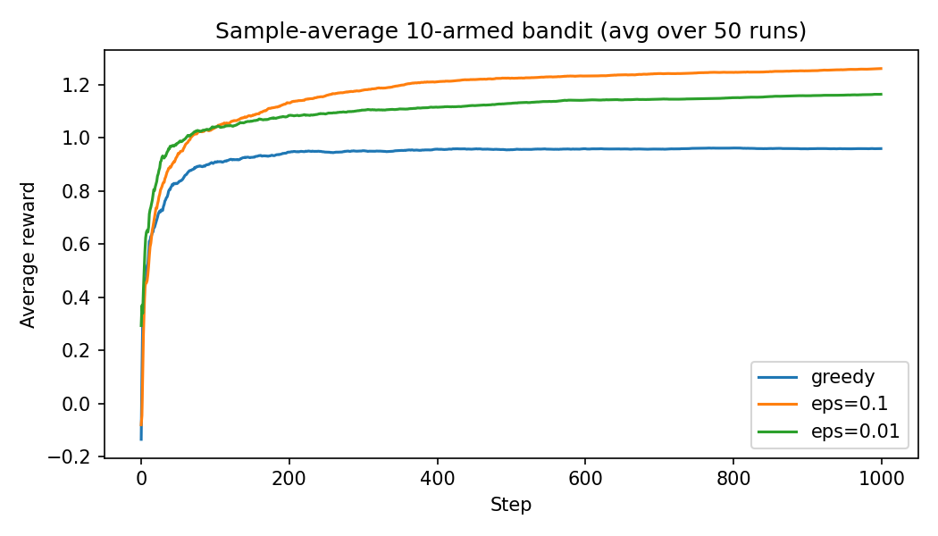 You can see that in the long run, the greedy method performs worse. There might be situations where greedy actions yield better results, because it can just find the optimal action and keep selecting that. But in more realistic scenarios, for example when the task is non-stationary, non-greedy actions are usually better, because they keep exploring the options.
Here is the Python code used for the example above (written by me, so it might contain mistakes):
You can see that in the long run, the greedy method performs worse. There might be situations where greedy actions yield better results, because it can just find the optimal action and keep selecting that. But in more realistic scenarios, for example when the task is non-stationary, non-greedy actions are usually better, because they keep exploring the options.
Here is the Python code used for the example above (written by me, so it might contain mistakes):
```Python title:’10-arm bandit’ fold import numpy as np import matplotlib.pyplot as plt
def run_bandit(n_arms: int = 10, steps: int = 1000, epsilon: float = 0.0, seed: int | None = None, true_means: np.ndarray | None = None): rng = np.random.default_rng(seed) if true_means is None: true_means = rng.normal(0.0, 1.0, size=n_arms) # Sample-average estimates and counts Q = np.zeros(n_arms) N = np.zeros(n_arms, dtype=int) rewards = np.empty(steps) for _ in range(steps): # Epsilon-greedy with random tie-breaking if rng.random() < epsilon: a = rng.integers(0, n_arms) else: max_val = Q.max() best_actions = np.flatnonzero(Q == max_val) a = rng.choice(best_actions) # Sample reward: R ~ N(q*(a), 1) r = rng.normal(true_means[a], 1.0) rewards[_] = r
# Incremental sample-average update N[a] += 1 Q[a] += (r - Q[a]) / N[a]
return rewards
if name == “main”: n_arms, steps = 10, 1000 num_runs = 50 labels_eps = [(0.0, “greedy”), (0.1, “eps=0.1”), (0.01, “eps=0.01”)] env_rng = np.random.default_rng(0)
# Accumulate per-step rewards over runs, then average sums = {eps: np.zeros(steps) for eps, _ in labels_eps} for run in range(num_runs): # New bandit instance each run (as in the 10-armed testbed) true_means = env_rng.normal(0.0, 1.0, size=n_arms) for i, (eps, _) in enumerate(labels_eps): rewards = run_bandit(n_arms=n_arms, steps=steps, epsilon=eps, seed=10_000 + run * 10 + i, true_means=true_means) sums[eps] += rewards plt.figure(figsize=(7, 4)) for eps, lbl in labels_eps: avg_rewards = sums[eps] / num_runs running_avg = np.cumsum(avg_rewards) / np.arrange(1, steps + 1) plt.plot(running_avg, lw=1.5, label=lbl) plt.xlabel(“Step”) plt.ylabel(“Average reward”) plt.title(f”Sample-average 10-armed bandit (avg over {num_runs} runs)”) plt.legend() plt.tight_layout() plt.savefig(“reward.png”, dpi=150) ```
Note that in practice, updating the estimates as introduced earlier usus a lot of memory. Instead incremental implementation is used.
\[Q_{k + 1} = Q_k\ +\ \frac{1}{k} (R_k\ -\ Q_k)\]Instead of $\frac{1}{k}$, other step sizes could also be used. For example, in a non-stationary problem, it makes sense to weight recent rewards more heavily than the older ones. One of the most popular methods of doing this is using a constant step-size parameter (similar to a forgetting factor used in recursive least square estimation in system identification or adaptive control).
\[Q_{k + 1} = Q_k\ +\ \alpha (R_k\ -\ Q_k) = (1 - \alpha)^k \ Q_1 + \sum_{i = 1}^{k} \alpha \ (1 \ -\ alpha)^{k - i} R_i\]This is sometimes called an exponential, recency-weighted average. A well-known result in stochastic approximation theory gives us the conditions required to assure convergence with probability 1:
\[\sum_{k = 1}^{\infty} \alpha_k (a) = \infty \quad\quad\quad \sum_{k = 1}^{\infty} \alpha_k^2 (a) < \infty\]The first condition is required to guarantee that the steps are large enough to eventually overcome any initial condition. The second condition guarantees that eventually the steps become small enough to assure convergence.
Optimistic Initial Values
The methods discuss so far depend on their initial values. These methods are biased by their initial estimates. For the sample-average methods, the bias disappears once all actions have been selected at least once, but for methods with constant $\alpha$, the bias is permanent, though decreasing over time. Initial action values not only can be used to some prior knowledge about what level of rewards can be expected, but can also be used as a simple way of encouraging exploration. When the initial action values are way too optimistically high, the agent starts by trying an action and gets disappointed after the actual reward it gets is lower than its estimate, so it goes on to try the other bandits, and so on. This method of encouraging exploration is called optimistic initial values. Note that this is just a simple trick. For example, it is not well suited to non-stationary problems because its drive for exploration is temporary.
Upper-Confidence-Bound Action Selection
As we saw, $\varepsilon$-greedy action selection forces the non-greedy actions to be tried, but indiscriminately. It would be better to select among the non-greedy actions according to their potential for actually being optimal. One effective way of doing this is to select the action as
\[A_t = arg \max_a \ (Q_t (a) + c \sqrt{\frac{\ln t}{N_t (a)}})\]The idea of this upper confidence bound (UCB) action selection is that the square-root term is a measure of the uncertainty or variance in the estimate of $a$’s value. Each time $a$ is selected the uncertainty is presumably reduced; $N_t (a)$ is incremented and, as it appears in the denominator of the uncertainty term, the term is decreased. UCB generally performs better that $\varepsilon$-greedy action selection, except in the first $n$ plays, when it selects randomly among the as-yet unplayed actions.
Gradient Bandits
Instead of estimating values and using those estimations to select actions, we can directly estimate preferences. The preference has no interpretation in terms of reward. Only the relative preference of one action over another is important; if we add $1000$ to all the preferences there is no affect on the action probabilities, which are determined according to a soft-max distribution as follows:
\[Pr \{ A_t = a \} = \frac{e^{H_t (a)}}{\sum_{b = 1}^{n} e^{H_t (b)}} = \pi_t (a)\]where $\pi_t (a)$ denotes the probability of selecting action $a$. Initially all preferences are the same. There is a natural learning algorithm for this setting based on the idea of stochastic gradient ascent. On each step, after selecting the action $A_t$ and receiving the reward $R_t$, the preferences are updated by:
\[H_{t + 1} (A_t) = H_t (A_t) + \alpha (R_t - \bar{R}_t) (1 - \pi_t (A_t))\] \[H_{t + 1} (a) = H_t (a) - \alpha (R_t - \bar{R}_t) \pi_t (a) \,\ \forall a \neq A_t\]$\bar{R}t$ is the average of all the rewards up through and including time $t$ and is called the _baseline. The choice of the baseline does not affect the expected update of the algorithm, but it does affect the variance of the update and thus the rate of convergence. Choosing it as the average of the rewards may not be the very best, but it is simple and works well in practice. The expected update of the gradient-bandit algorithm is equal to the gradient of expected reward, and thus that the algorithm is an instance of stochastic gradient ascent.
Associative Search
Up to this point, we have considered only non-associative tasks, in which there is no need to associate different actions with different situations. However, in a general reinforcement learning task there is more than one situation, and the goal is to learn a policy: a mapping from situations to the actions that are best in those situations. An associative search task includes remembering the situation you are facing and remembering different mappings for them. It is so called because it involves both trial-and-error learning in the form of search for the best actions and association of these actions with the situations in which they are best.
To learn more about reinforcement learning, continue to Finite Markov Decision Processes.
Sources: