Finite Markov Decision Processes
#RL #Learning #computer-science #Control
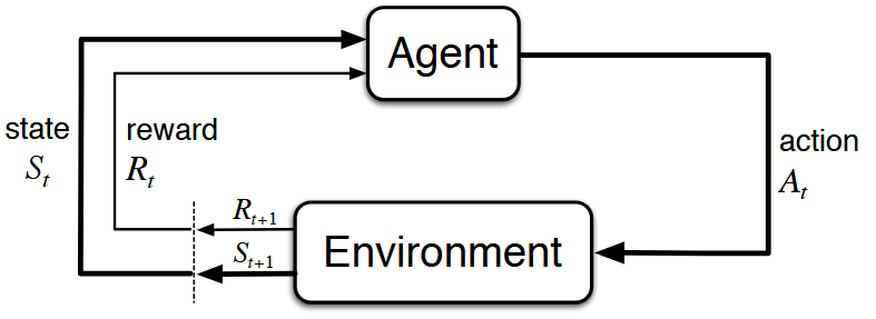
The reinforcement learning problem is meant to be a straightforward framing of the problem of learning from interaction to achieve a goal. The learner and decision-maker is called the agent. The thing it interacts with, comprising everything outside the agent, is called the environment.
A complete specification of an environment defines a task , one instance of the reinforcement learning problem. More specifically, the agent and environment interact at each of a sequence of discrete time steps, $t = 0, 1, 2, 3, \cdot\cdot\cdot$ , the agent receives some representation of the environment’s state, $S_t \in \mathcal{S}$, where $\mathcal{S}$ is the set of possible states, and on that basis selects an action, $A_t \in \mathcal{A} (S_t)$, where $\mathcal{A} (S_t)$ is the set of actions available in state $S_t$. One time step later, in part as a consequence of its action, the agent receives a numerical reward , $R_{t + 1} \in \mathcal{R} \subset \mathbb{R}$ , and finds itself in a new state, $S_{t + 1}$.
 At each time step, the agent implements a mapping from states to probabilities of selecting each possible action. This mapping is called the agent’s policy and is denoted $\pi_t$, where $\pi_t (a | s)$ is the probability that $A_t = a$ if $S_t = s$.
The boundary between the agent and the environment is important. As a general rule, anything that cannot be changed arbitrarily by the agent is considered to be outside of it and thus part of its environment. The agent-environment boundary represents the limit of the agent’s absolute control, not of its knowledge.
The reinforcement learning framework is a considerable abstraction of the problem of goal-directed learning from interaction. It proposes that any problem of learning goal-directed behavior can be reduced to three signals passing back and forth between an agent and its environment:
At each time step, the agent implements a mapping from states to probabilities of selecting each possible action. This mapping is called the agent’s policy and is denoted $\pi_t$, where $\pi_t (a | s)$ is the probability that $A_t = a$ if $S_t = s$.
The boundary between the agent and the environment is important. As a general rule, anything that cannot be changed arbitrarily by the agent is considered to be outside of it and thus part of its environment. The agent-environment boundary represents the limit of the agent’s absolute control, not of its knowledge.
The reinforcement learning framework is a considerable abstraction of the problem of goal-directed learning from interaction. It proposes that any problem of learning goal-directed behavior can be reduced to three signals passing back and forth between an agent and its environment:
- one signal to represent the choices made by the agent (the actions)
- one signal to represent the basis on which the choices are made (the states)
- one signal to define the agent’s goal (the rewards). Remember that rewards are always single numbers.
Goals and Rewards
The reward hypothesis states that
[!definition] All of what we mean by goals and purposes can be well thought of as the maximization of the expected value of the cumulative sum of a received scalar signal called reward.
In particular, this means that the reward signal is not the place to impart to the agent prior knowledge about how to achieve what we want it to do. The reward should contain all the information necessary for the learner to know what it wants to achieve. Another important thing is that the rewards are computed in the environment rather than in the agent.
Returns
But what aspect of the reward are we trying to maximize? Because we know that increasing immediate reward doesn’t necessarily mean that the future rewards will be increased as well. In general, we seek to maximize the expected return, where the return $G_t$ is defined as some specific function of the reward sequence. In the simplest case, we might define \(G_t = R_{t + 1} + R_{t + 2} + \cdot\cdot\cdot +R_T\) where $T$ is a final time step. This approach makes sense in applications in which there is a natural notion of final time step, that is, when the agent-environment interaction breaks naturally into subsequences, which we call episodes, Each episode ends in a special state called the terminal state, followed by a reset to a standard starting state or to a sample from a standard distribution of starting states. Tasks with episodes of this kind are called episodic tasks. In episodic tasks we sometimes need to distinguish the set of all nonterminal states, denoted $\mathcal{S}$, from the set of all states plus the terminal state, denoted $\mathcal{S}^+$. On the other hand, in many cases the agent–environment interaction does not break naturally into identifiable episodes, but goes on continually without limit. These are called continuous tasks. The return function we defined earlier would pose problems where $T \rightarrow \infty$. Therefore, we define the notion of discounting. In particular, the agent can be though to be choosing $A_t$ to maximize \(G_t = R_{t + 1} + \gamma R_{t + 2} + \gamma^2 R_{t + 3} + \cdot\cdot\cdot = \sum_{k = 0}^{\infty} \gamma^k R_{t + k + 1}\) where $0 \leq \gamma \leq 1$ is a parameter called the discount rate. If $\gamma < 1$, the infinite sum has a finite value as long as the reward sequence ${R_k}$ is bounded To unify the notation for episodic and continuous tasks, episode termination can be considered to be the entering of a special absorbing state that transitions only to itself and that generates only rewards of zero. Therefore, in general, we can consider the return to be \(G_t = \sum_{k = 0}^{T - t - 1} \gamma^k R_{t + k + 1}\) including the possibility that $T = \infty$ or $\gamma = 1$, but not both.
Markov Property
In the field of RL, unlike in control theory, state refers to whatever information that is available to the agent. A state signal that succeeds in retaining all relevant information is said to be Markov, or to have the Markov property. In the general case, the dynamics of the environment can be defined by specifying the complete probability distribution \(Pr \{ R_{t + 1} = r, S_{t + 1} = s' \ | \ S_0, A_0, R_1, \cdot\cdot\cdot S_{t - 1}, A_{t - 1}, R_t, S_t, A_t \}\)but if the state signal has the Markov property, the environment’s response at $t + 1$ depends only on the state and action representations at $t$ and thus can be defined by specifying only \(p(s', r \ | \ s, a) = Pr \{ R_{t + 1} = r, S_{t + 1} = s' \ | \ S_t, A_t \}\) In reality, due to presence of noise, disturbances and other random events that cannot necessarily be considered, it is useful to think of the state at each time step as an approximation to a Markov state, although it may not fully satisfy the Markov property.
Markov Decision Processes
A reinforcement learning task that satisfies the Markov property is called a Markov decision process, or MDP. If the state and action spaces are finite, then it is called a finite Markov decision process (finite MDP). By specifying the dynamics of the environment as we did here, one can compute anything else one might want to know about the environment, such as the expected rewards for state-action pairs: \(r(s, a) = \mathbb{E} \{ R_{t + 1} \ | \ S_t = s, A_t = a \} = \sum_{r \ in \mathcal{R}} r \sum_{s' \ in \mathcal{S}} p(s', r \ | \ s, a)\) the state-transition probabilities: \(p(s' \ | \ s,a) = Pr \{ S_{t + 1} = s' \ | \ S_t = s, A_t = a \} = \sum_{r \in \mathcal{R}} p(s', r \ | \ s, a)\)
Value Functions
A policy, $\pi$, is a mapping from each state, $s \in \mathcal{S}$, and action, $a \in \mathcal{A} (s)$, to the probability $\pi ( a \ | \ s)$ of taking action $a$ when in state $s$. Informally, the value of a state $s$ under a policy $\pi$, denoted $v_\pi (s)$, is the expected return when starting in $s$ and following $\pi$ thereafter. For MDPs, we can define $v_\pi (s)$ formally as \(v_\pi (s) = \mathbb{E} [G_t \ | \ S_t = s] = \mathbb{E}_\pi [\sum_{k = 0}^{\infty} \gamma^k R_{t + k + 1} \ | \ S_t = s]\) We call the function $v_\pi$ the state-value function for policy $\pi$. The value of the terminal state, if any, is always zero.
Similarly, we define the value of taking action $a$ in state $s$ under a policy $\pi$, denoted $q_\pi (s, a)$, as the expected return starting from $s$, taking the action $a$, and thereafter following policy $\pi$: \(q_\pi (s, a)= \mathbb{E}_\pi [G_t \ | \ S_t = s, A_t = a] = \mathbb{E} [\sum_{k = 0}^{\infty} \gamma^k R_{t + k + 1} \ | \ S_t = s, A_t = a]\) We call $q_\pi$ the action-value function for policy $\pi$. The value functions $v_\pi$ and $q_\pi$ can be estimated from experience.
The bellman equation for $v_\pi$ can be written as \(v_\pi (s) = \sum_a \pi (a \ | \ s) \sum_{s', r} p(s', r \ | \ s, a) [r + \gamma v_\pi (s')]\) The value function $v_\pi$ is the unique solution to its Bellman equation.
Optimal Value Functions
A policy $\pi$ is defined to be better than or equal to a policy $\pi’$ if its expected return is greater than or equal to that of $\pi’$ for all states. In other words, $\pi \geq \pi’$ if and only if $v_\pi (s) \geq v_\pi’ (s)$ for all $s \in \mathcal{S}$. There is always at least one policy that is better than or equal to all other policies. This is an optimal policy. The optimal policy may not be unique. All optimal policies share the same state-value function, called the optimal state-value function, denoted by $v_{\pi^\ast}$, and defined as \(v_\ast (s) = \max_\pi v_\pi (s)\) for all $s \in \mathcal{S}$. Optimal policies also share the same optimal action-value function, denoted $q_\ast$, and defined as \(q_\ast = \mathbb{E} [R_{t + 1} + \gamma v_\ast (S_{t + 1)}) \ | \ S_t = s, A_t = a]\)
The Bellman optimality equation expresses the fact that the value of a state under an optimal policy must equal the expected return for the best action from that state. It can be written as \(v_\ast (s) = \max_a \mathbb{E} [R_{t + 1} + \gamma v_\ast (S_{t+1}) \ | \ S_t = s, A_t = a] = \max_{a \in \mathcal{A}} \sum_{s', r} p(s', r \ | \ s, a)[r + \gamma v_\ast (s')]\) The bellman optimality equation for $q_\ast$ is \(q_\ast (s, a) = \mathbb{E} [R_{t + 1} + \gamma \max_{a'} q_\ast (S_{t + 1}, a') \ | \ S_t = s, A_t = a] = \sum_{s', r} p(s', r \ | \ s, a) [r + \max_{a'} q_\ast (s', a')]\) For finite MDPs, the Bellman optimality equation has a unique solution independent of the policy. The Bellman optimality equation is actually a system of equations, one for each state. If the dynamics of the environment are known $p(s’, r \ | \ s, a)$, then in principle one can solve this system of equations. However, the solution relies on at least three assumptions that are rarely true in practice:
- We accurately know the dynamics of the environment
- We have enough computational resources to complete the computation of the solution
- The Markov property Therefore, many RL algorithms approximate the solution to the Bellman optimality equation.
Any policy that is greedy with respect to the optimal evaluation function $v_\ast$ is an optimal policy.
Continue reading about reinforcement learning here.
Sources: